
LFSR – Linear Feedback Shift Register
LFSR logic is commonly used in hardware and software to generate pseudo-random data. An n-bit LFSR cycles between as many as 2^n - 1 unique, non-zero states.
In some contexts, the output of the LFSR is considered a single bit, the state of the right-most register in these examples. In other situations, the output is the state of all of the registers.
Two configurations are possible: Galois (also known as type 2), and Fibonacci (also known as type 1). The single bit output at the right-most register is identical for both configurations. The output at the other bit positions differ, but only by a time delay. The time delay for each bit position can be found by inspection for the Fibonacci configuration, and with a calculation for the Galois configuration, as shown below.
Both Galois and Fibonacci configurations can be drawn with left shifting registers or right shifting registers. But the choice of shift direction is not important. Because no inherently directional operation such as carry propagation is involved, the operation of the two mirror each other. The shift direction used here has been chosen to accommodate comparing the Galois and Fibonacci configurations.
Galois configuration for polynomial x^10 + x^3 + 1
The state of the LFSR at time t can be written in terms of the previous state. The equations are found by inspection of the circuit:
 g0 (t) = g9 (t-1)            (1)
 g1 (t) = g0 (t-1)
 g2 (t) = g1 (t-1)
 g3 (t) = g2 (t-1) ^ g9(t-1)
 g4 (t) = g3 (t-1)
 g5 (t) = g4 (t-1)
 g6 (t) = g5 (t-1)
 g7 (t) = g6 (t-1)
 g8 (t) = g7 (t-1)
 g9 (t) = g8 (t-1)
In matrix form, the current state is multiplied by the matrix to give the next state. Each bit in the current state selects a row in the matrix. The selected rows are exclusive ored together to produce the next state.
  0000000010
  0000000100
  0000001000
  0000010000
  0000100000
  0001000000
  0010000000
  0100000000
  1000000000
  0000001001
Fibonacci configuration for polynomial x^10 + x^3 + 1
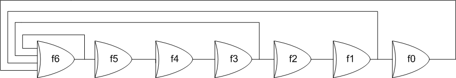
The state of the LFSR at time t can be written in terms of the previous state. The equations are found by inspection of the circuit:
 f0 (t) = f1 (t-1)              (2)
 f1 (t) = f2 (t-1)
 f2 (t) = f3 (t-1)
 f3 (t) = f4 (t-1)
 f4 (t) = f5 (t-1)
 f5 (t) = f6 (t-1)
 f6 (t) = f7 (t-1)
 f7 (t) = f8 (t-1)
 f8 (t) = f9 (t-1)
 f9 (t) = f0 (t-1)  ^ f3 (t-1)
The next state matrix for the Fibonacci configuration:
  1000000000
  0000000001
  0000000010
  1000000100
  0000001000
  0000010000
  0000100000
  0001000000
  0010000000
  0100000000
The next state matrix of one LFSR configuration is the transpose of the next state matrix of the other configuration.
The LFSRs cycle through the following states when the registers are initially loaded with 0000000001:
Galois Fibonacci
t     g9······g0   f9······f0
0     0000000001   0000000001
1     0000000010   1000000000
2     0000000100   0100000000
3     0000001000   0010000000
4     0000010000   0001000000
5     0000100000   0000100000
6     0001000000   0000010000
7     0010000000   0000001000
8     0100000000   1000000100
9     1000000000   0100000010
10    0000001001   0010000001
11    0000010010   1001000000
12    0000100100   0100100000
13    0001001000   0010010000
14    0010010000   0001001000
15    0100100000   1000100100

        (complete listing)
1007  1001011101   0011010011
1008  0010110011   1001101001
1009  0101100110   0100110100
1010  1011001100   0010011010
1011  0110010001   1001001101
1012  1100100010   0100100110
1013  1001001101   0010010011
1014  0010010011   1001001001
1015  0100100110   0100100100
1016  1001001100   0010010010
1017  0010010001   0001001001
1018  0100100010   0000100100
1019  1001000100   0000010010
1020  0010000001   0000001001
1021  0100000010   0000000100
1022  1000000100   0000000010
<cycle repeats starting here>
Equivalence of Galois and Fibonacci configurations for polynomial x^10 + x^3 + 1
Notice that the output, when taken as the single right-most register, is the same for both configurations. This is true in general, and can be demonstrated by writing the output equations for the right-most register of both configurations in terms of previous values of the register. For the Fibonacci configuration, start with equations (2) and solve for f0 (t) as a function of f0 at times t-1 through t-10:
f0 (t) = f1 (t-1)
f0 (t) = f2 (t-2)
f0 (t) = f3 (t-3)
f0 (t) = f4 (t-4)
f0 (t) = f5 (t-5)
f0 (t) = f6 (t-6)
f0 (t) = f7 (t-7)
f0 (t) = f8 (t-8)
f0 (t) = f9 (t-9)
f0 (t) = f0 (t-10) ^ f3 (t-10)
f0 (t) = f0 (t-10) ^ f0 (t-7)

f1 (t) = f0 (t+1)
       = f0 (t-9) ^ f0 (t-6)

f2 (t) = f0 (t+2)
       = f0 (t-8) ^ f0 (t-5)

f3 (t) = f0 (t+3)
       = f0 (t-7) ^ f0 (t-4)

f4 (t) = f0 (t+4)
       = f0 (t-6) ^ f0 (t-3)

f5 (t) = f0 (t+5)
       = f0 (t-5) ^ f0 (t-2)

f6 (t) = f0 (t+6)
       = f0 (t-4) ^ f0 (t-1)

f7 (t) = f0 (t+7)
       = f0 (t-3) ^ f0 (t-0)
       = f0 (t-3) ^ f0 (t-10) ^ f0 (t-7)

f8 (t) = f0 (t+8)
       = f0 (t-2) ^ f0 (t+1)
       = f0 (t-2) ^ f0 (t-9) ^ f0 (t-6)

f9 (t) = f0 (t+9)
       = f0 (t-1) ^ f0 (t+2)
       = f0 (t-1) ^ f0 (t-8) ^ f0 (t5)

 f0 (t) = f0 (t-10) ^ f0 (t-7)             (3)
 f1 (t) = f0 (t-9)  ^ f0 (t-6)
 f2 (t) = f0 (t-8)  ^ f0 (t-5)
 f3 (t) = f0 (t-7)  ^ f0 (t-4)
 f4 (t) = f0 (t-6)  ^ f0 (t-3)
 f5 (t) = f0 (t-5)  ^ f0 (t-2)
 f6 (t) = f0 (t-4)  ^ f0 (t-1)
 f7 (t) = f0 (t-10) ^ f0 (t-7) ^ f0 (t-3)
 f8 (t) = f0 (t-9)  ^ f0 (t-6) ^ f0 (t-2)
 f9 (t) = f0 (t-8)  ^ f0 (t-5) ^ f0 (t-1)

The coefficients for the terms in the above
equations can also be found with a calculation:
    t-1···t-10        calculation    p10······p0 p9······p0
f0  0000001001        gf2util modmul,10000001001,0000001001,1
f1  0000010010        gf2util modmul,10000001001,0000001001,10
f2  0000100100        gf2util modmul,10000001001,0000001001,100
f3  0001001000        gf2util modmul,10000001001,0000001001,1000
f4  0010010000        gf2util modmul,10000001001,0000001001,10000
f5  0100100000        gf2util modmul,10000001001,0000001001,100000
f6  1001000000        gf2util modmul,10000001001,0000001001,1000000
f7  0010001001        gf2util modmul,10000001001,0000001001,10000000
f8  0100010010        gf2util modmul,10000001001,0000001001,100000000
f9  1000100100        gf2util modmul,10000001001,0000001001,1000000000

For the Galois configuration, start with equations (1) and solve for g0 (t) as a function of g0 at times t-1 through t-10:
g0 (t) = g9 (t-1)
g1 (t) = g0 (t-1)
g2 (t) = g1 (t-1)
g3 (t) = g2 (t-1) ^ g9 (t-1)
g4 (t) = g3 (t-1)
g5 (t) = g4 (t-1)
g6 (t) = g5 (t-1)
g7 (t) = g6 (t-1)
g8 (t) = g7 (t-1)
g9 (t) = g8 (t-1)

g0 (t) = g9 (t-1)
g1 (t) = g0 (t-1)
g2 (t) = g0 (t-2)
g3 (t) = g2 (t-1) ^ g9 (t-1)
g4 (t) = g3 (t-1)
g5 (t) = g4 (t-1)
g6 (t) = g5 (t-1)
g7 (t) = g6 (t-1)
g8 (t) = g7 (t-1)
g9 (t) = g8 (t-1)

g0 (t) = g9 (t-1)
g1 (t) = g0 (t-1)
g2 (t) = g0 (t-2)
g3 (t) = g2 (t-1) ^ g0 (t)
g4 (t) = g3 (t-1)
g5 (t) = g4 (t-1)
g6 (t) = g5 (t-1)
g7 (t) = g6 (t-1)
g8 (t) = g7 (t-1)
g9 (t) = g8 (t-1)

g0 (t) = g9 (t-1)
g1 (t) = g0 (t-1)
g2 (t) = g0 (t-2)
g3 (t) = g0 (t-3) ^ g0 (t)
g4 (t) = g3 (t-1)
g5 (t) = g4 (t-1)
g6 (t) = g5 (t-1)
g7 (t) = g6 (t-1)
g8 (t) = g7 (t-1)
g9 (t) = g8 (t-1)

g0 (t) = g9 (t-1)
g1 (t) = g0 (t-1)
g2 (t) = g0 (t-2)
g3 (t) = g0 (t-3) ^ g0 (t)
g4 (t) = g0 (t-4) ^ g0 (t-1)
g5 (t) = g4 (t-1)
g6 (t) = g5 (t-1)
g7 (t) = g6 (t-1)
g8 (t) = g7 (t-1)
g9 (t) = g8 (t-1)

g0 (t) = g9 (t-1)
g1 (t) = g0 (t-1)
g2 (t) = g0 (t-2)
g3 (t) = g0 (t-3) ^ g0 (t)
g4 (t) = g0 (t-4) ^ g0 (t-1)
g5 (t) = g0 (t-5) ^ g0 (t-2)
g6 (t) = g5 (t-1)
g7 (t) = g6 (t-1)
g8 (t) = g7 (t-1)
g9 (t) = g8 (t-1)

g0 (t) = g9 (t-1)
g1 (t) = g0 (t-1)
g2 (t) = g0 (t-2)
g3 (t) = g0 (t-3) ^ g0 (t)
g4 (t) = g0 (t-4) ^ g0 (t-1)
g5 (t) = g0 (t-5) ^ g0 (t-2)
g6 (t) = g0 (t-6) ^ g0 (t-3)
g7 (t) = g6 (t-1)
g8 (t) = g7 (t-1)
g9 (t) = g8 (t-1)

g0 (t) = g9 (t-1)
g1 (t) = g0 (t-1)
g2 (t) = g0 (t-2)
g3 (t) = g0 (t-3) ^ g0 (t)
g4 (t) = g0 (t-4) ^ g0 (t-1)
g5 (t) = g0 (t-5) ^ g0 (t-2)
g6 (t) = g0 (t-6) ^ g0 (t-3)
g7 (t) = g0 (t-7) ^ g0 (t-4)
g8 (t) = g7 (t-1)
g9 (t) = g8 (t-1)

g0 (t) = g9 (t-1)
g1 (t) = g0 (t-1)
g2 (t) = g0 (t-2)
g3 (t) = g0 (t-3) ^ g0 (t)
g4 (t) = g0 (t-4) ^ g0 (t-1)
g5 (t) = g0 (t-5) ^ g0 (t-2)
g6 (t) = g0 (t-6) ^ g0 (t-3)
g7 (t) = g0 (t-7) ^ g0 (t-4)
g8 (t) = g0 (t-8) ^ g0 (t-5)
g9 (t) = g8 (t-1)

g0 (t) = g9 (t-1)
g1 (t) = g0 (t-1)
g2 (t) = g0 (t-2)
g3 (t) = g0 (t-3) ^ g0 (t)
g4 (t) = g0 (t-4) ^ g0 (t-1)
g5 (t) = g0 (t-5) ^ g0 (t-2)
g6 (t) = g0 (t-6) ^ g0 (t-3)
g7 (t) = g0 (t-7) ^ g0 (t-4)
g8 (t) = g0 (t-8) ^ g0 (t-5)
g9 (t) = g0 (t-9) ^ g0 (t-6)

g0 (t) = g0 (t-10) ^ g0 (t-7)
g1 (t) = g0 (t-1)
g2 (t) = g0 (t-2)
g3 (t) = g0 (t-3) ^ g0 (t)
g4 (t) = g0 (t-4) ^ g0 (t-1)
g5 (t) = g0 (t-5) ^ g0 (t-2)
g6 (t) = g0 (t-6) ^ g0 (t-3)
g7 (t) = g0 (t-7) ^ g0 (t-4)
g8 (t) = g0 (t-8) ^ g0 (t-5)
g9 (t) = g0 (t-9) ^ g0 (t-6)

g0 (t) = g0 (t-10) ^ g0 (t-7)
g1 (t) = g0 (t-1)
g2 (t) = g0 (t-2)
g3 (t) = g0 (t-3) ^ g0 (t-10) ^ g0 (t-7)
g4 (t) = g0 (t-4) ^ g0 (t-1)
g5 (t) = g0 (t-5) ^ g0 (t-2)
g6 (t) = g0 (t-6) ^ g0 (t-3)
g7 (t) = g0 (t-7) ^ g0 (t-4)
g8 (t) = g0 (t-8) ^ g0 (t-5)
g9 (t) = g0 (t-9) ^ g0 (t-6)

 g0 (t) = g0 (t-10) ^ g0 (t-7)             (4)
 g1 (t) = g0 (t-1)
 g2 (t) = g0 (t-2)
 g3 (t) = g0 (t-10) ^ g0 (t-7) ^ g0 (t-3)
 g4 (t) = g0 (t-4)  ^ g0 (t-1)
 g5 (t) = g0 (t-5)  ^ g0 (t-2)
 g6 (t) = g0 (t-6)  ^ g0 (t-3)
 g7 (t) = g0 (t-7)  ^ g0 (t-4)
 g8 (t) = g0 (t-8)  ^ g0 (t-5)
 g9 (t) = g0 (t-9)  ^ g0 (t-6)
The coefficients for the terms in the above equations can also be found with a calculation:
    t-1···t-10                      p10······p0
g1  1000000000       gf2util modmul,10000001001,01000000000,1
g2  0100000000       gf2util modmul,10000001001,00100000000,1
g3  0010001001       gf2util modmul,10000001001,10010000000,1
g4  1001000000       gf2util modmul,10000001001,01001000000,1
g5  0100100000       gf2util modmul,10000001001,00100100000,1
g6  0010010000       gf2util modmul,10000001001,00010010000,1
g7  0001001000       gf2util modmul,10000001001,00001001000,1
g8  0000100100       gf2util modmul,10000001001,00000100100,1
g9  0000010010       gf2util modmul,10000001001,00000010010,1
g0  0000001001       gf2util modmul,10000001001,00000001001,1
The above shows that for the LFSR using polynomial x^10 + x^3 + 1, the output of the right-most register is the same for both the Galois and Fibonacci configurations.
Converting a Fibonacci state to the corresponding Galois state

To convert a Fibonacci state into the corresponding Galois state, the equations for the Galois state must be written in terms of the current Fibonacci state, f0 (t) through f6(t).

The current Fibonacci state holds future register zero states:
f0 (t) = f0 (t+0)
f1 (t) = f0 (t+1)
f2 (t) = f0 (t+2)
f3 (t) = f0 (t+3)
f4 (t) = f0 (t+4)
f5 (t) = f0 (t+5)
f6 (t) = f0 (t+6)
f7 (t) = f0 (t+7)
f8 (t) = f0 (t+8)
f9 (t) = f0 (t+9)

Start with equations (4) and write the Galois state in terms of future register zero states
 g0 (t) = g0 (t-10) ^ g0 (t-7)
 g1 (t) = g0 (t-1)
 g2 (t) = g0 (t-2)
 g3 (t) = g0 (t-10) ^ g0 (t-7) ^ g0 (t-3)
 g4 (t) = g0 (t-4)  ^ g0 (t-1)
 g5 (t) = g0 (t-5)  ^ g0 (t-2)
 g6 (t) = g0 (t-6)  ^ g0 (t-3)
 g7 (t) = g0 (t-7)  ^ g0 (t-4)
 g8 (t) = g0 (t-8)  ^ g0 (t-5)
 g9 (t) = g0 (t-9)  ^ g0 (t-6)

Equations used to shift t-10 through t-1 references to t+0 through t+9:
0 = g0 (t-10) ^ g0 (t-7) ^ g0 (t+0)
0 = g0 (t-9)  ^ g0 (t-6) ^ g0 (t+1)
0 = g0 (t-8)  ^ g0 (t-5) ^ g0 (t+2)
0 = g0 (t-7)  ^ g0 (t-4) ^ g0 (t+3)
0 = g0 (t-6)  ^ g0 (t-3) ^ g0 (t+4)
0 = g0 (t-5)  ^ g0 (t-2) ^ g0 (t+5)
0 = g0 (t-4)  ^ g0 (t-1) ^ g0 (t+6)
0 = g0 (t-3)  ^ g0 (t+0) ^ g0 (t+7)
0 = g0 (t-2)  ^ g0 (t+1) ^ g0 (t+8)
0 = g0 (t-1)  ^ g0 (t+2) ^ g0 (t+9)

g1 (t) = g0 (t-1)
       = g0 (t-1)  ^ g0 (t-1) ^ g0 (t+2) ^ g0 (t+9)
       = g0 (t+2)  ^ g0 (t+9)

g2 (t) = g0 (t-2)
       = g0 (t-2)  ^ g0 (t-2)  ^ g0 (t+1) ^ g0 (t+8)
       = g0 (t+1)  ^ g0 (t+8)

g3 (t) = g0 (t-10) ^ g0 (t-7) ^ g0 (t-3)
       = g0 (t-10) ^ g0 (t-7) ^ g0 (t-3) ^ g0 (t-10) ^ g0 (t-7) ^ g0 (t+0)
       = g0 (t-3)  ^ g0 (t+0)
       = g0 (t-3)  ^ g0 (t+0) ^ g0 (t-3)  ^ g0 (t+0) ^ g0 (t+7)
       = g0 (t+7)

g4 (t) = g0 (t-4)  ^ g0 (t-1)
       = g0 (t-4)  ^ g0 (t-1) ^ g0 (t-4)  ^ g0 (t-1) ^ g0 (t+6)
       = g0 (t+6)

g5 (t) = g0 (t-5)  ^ g0 (t-2)
       = g0 (t-5)  ^ g0 (t-2) ^ g0 (t-5)  ^ g0 (t-2) ^ g0 (t+5)
       = g0 (t+5)

g6 (t) = g0 (t-6)  ^ g0 (t-3)
       = g0 (t-6)  ^ g0 (t-3) ^ g0 (t-6)  ^ g0 (t-3) ^ g0 (t+4)
       = g0 (t+4)

g7 (t) = g0 (t-7)  ^ g0 (t-4)
       = g0 (t-7)  ^ g0 (t-4) ^ g0 (t-7)  ^ g0 (t-4) ^ g0 (t+3)
       = g0 (t+3)

g8 (t) = g0 (t-8)  ^ g0 (t-5)
       = g0 (t-8)  ^ g0 (t-5) ^ g0 (t-8)  ^ g0 (t-5) ^ g0 (t+2)
       = g0 (t+2)

g9 (t) = g0 (t-9)  ^ g0 (t-6)
       = g0 (t-9)  ^ g0 (t-6) ^ g0 (t-9)  ^ g0 (t-6) ^ g0 (t+1)
       = g0 (t+1)

g0 (t) = g0 (t)
g1 (t) = g0 (t+2)  ^ g0 (t+9)
g2 (t) = g0 (t+1)  ^ g0 (t+8)
g3 (t) = g0 (t+7)
g4 (t) = g0 (t+6)
g5 (t) = g0 (t+5)
g6 (t) = g0 (t+4)
g7 (t) = g0 (t+3)
g8 (t) = g0 (t+2)
g9 (t) = g0 (t+1)
g0 (t) = f0 (t)
g1 (t) = f0 (t+2)  ^ f0 (t+9)
g2 (t) = f0 (t+1)  ^ f0 (t+8)
g3 (t) = f0 (t+7)
g4 (t) = f0 (t+6)
g5 (t) = f0 (t+5)
g6 (t) = f0 (t+4)
g7 (t) = f0 (t+3)
g8 (t) = f0 (t+2)
g9 (t) = f0 (t+1)

g0 (t) = f0 (t)            (5)
g1 (t) = f2 (t)  ^ f9 (t)
g2 (t) = f1 (t)  ^ f8 (t)
g3 (t) = f7 (t)
g4 (t) = f6 (t)
g5 (t) = f5 (t)
g6 (t) = f4 (t)
g7 (t) = f3 (t)
g8 (t) = f2 (t)
g9 (t) = f1 (t)
The coefficients for the terms in the above equations can also be found with a calculation involving the polynomial and coefficients from equations (4):
    f0······f9                      p0······p10 t-10···t-1
g0  1000000000       gf2util modmul,10010000001,1001000000,10000000000
g1  0010000001       gf2util modmul,10010000001,0000000001,10000000000
g2  0100000010       gf2util modmul,10010000001,0000000010,10000000000
g3  0000000100       gf2util modmul,10010000001,1001000100,10000000000
g4  0000001000       gf2util modmul,10010000001,0000001001,10000000000
g5  0000010000       gf2util modmul,10010000001,0000010010,10000000000
g6  0000100000       gf2util modmul,10010000001,0000100100,10000000000
g7  0001000000       gf2util modmul,10010000001,0001001000,10000000000
g8  0010000000       gf2util modmul,10010000001,0010010000,10000000000
g9  0100000000       gf2util modmul,10010000001,0100100000,10000000000
g0 (t) = f0 (t)
g1 (t) = f2 (t) ^ f9 (t)
g2 (t) = f1 (t) ^ f8 (t)
g3 (t) = f7 (t)
g4 (t) = f6 (t)
g5 (t) = f5 (t)
g6 (t) = f4 (t)
g7 (t) = f3 (t)
g8 (t) = f2 (t)
g9 (t) = f1 (t)
f0 (t) = g0 (t)
f1 (t) = g9 (t)
f2 (t) = g8 (t)
f3 (t) = g7 (t)
f4 (t) = g6 (t)
f5 (t) = g5 (t)
f6 (t) = g4 (t)
f7 (t) = g3 (t)
f8 (t) = g2 (t) ^ f1 (t)
       = g2 (t) ^ g9 (t)
f9 (t) = g1 (t) ^ f2 (t)
       = g1 (t) ^ g8 (t)
f0 (t) = g0 (t)           (6)
f1 (t) = g9 (t)
f2 (t) = g8 (t)
f3 (t) = g7 (t)
f4 (t) = g6 (t)
f5 (t) = g5 (t)
f6 (t) = g4 (t)
f7 (t) = g3 (t)
f8 (t) = g2 (t) ^ g9 (t)
f9 (t) = g1 (t) ^ g8 (t)

The coefficients for the terms in the above equations can also be found with a calculation involving the polynomial:
    g0······g9
f0  1000000000                               p10·····p1
f1  0000000001     gf2util divide,1000000000,1000000100
f2  0000000010     gf2util divide,10000000000,1000000100
f3  0000000100     gf2util divide,100000000000,1000000100
f4  0000001000     gf2util divide,1000000000000,1000000100
f5  0000010000     gf2util divide,10000000000000,1000000100
f6  0000100000     gf2util divide,100000000000000,1000000100
f7  0001000000     gf2util divide,1000000000000000,1000000100
f8  0010000001     gf2util divide,10000000000000000,1000000100
f9  0100000010     gf2util divide,100000000000000000,1000000100
Finding the time delay between LFSR stages
It can be seen from inspection of the circuit that the output of each Fibonacci stage differs from the output of a neighboring stage by one clock. But for the Galois configuration, the relationship as simple. A brute force approach for finding the delay for a register in the Galois configuration is to solve for each possible delay until one is found that is in the form of a single g0 term.
g1 (t) = g0 (t-1)
g2 (t) = g0 (t-2)
g3 (t) = g0 (t-1016)
g4 (t) = g0 (t-1017)
g5 (t) = g0 (t-1018)
g6 (t) = g0 (t-1019)
g7 (t) = g0 (t-1020)
g8 (t) = g0 (t-1021)
g9 (t) = g0 (t-1022)