This program implements the software described by the paper
Computer Model
Clarifies Spontaneous Charge Redistribution in Conductors. It currently builds
for Windows only, though porting to other operating systems should be easy. The
program is coded in C99 and builds with GCC, CLANG, or Microsoft build tools.
CLANG produces the best optimization, at least for an AMD Ryzen gen 1 processor.
The program input is a graphic file containing a 2-dimensional drawing of a
conductor. Save the file in BMP format, using white background with black for
the conductor portion. Suggested dimension is width 1600 pixels and height 1200
pixels. The included sample BMP graphic files were created using Microsoft
Paint.
Execute the program with no command line to see a description of the required
and optional parameters, along with default values:
staticCharge 1.0
use: staticCharge [options]
options:
bmp=<file path>
get conductor shape from this black on white image
charges=n
add n charges to conductor interior (default 500)
chargeloc=x,y
BMP file coordinate for adding charges (default: center)
chargesperpixel=f
density of added charges, default 1.00
pngfilter=n
write a png file every n cycles (default: 1B/(chargecount^2)
constant=f
set constant to f (default 0.005)
fieldalways
field lines for all PNGs, otherwise last only
fieldonly
plot the field lines and then exit
markmaxfield
mark surface position of max field when drawing field lines
periodicpngs
write PNG file snapshots periodically (to observe progress)
fieldradius=n
radius multiple for field line start (default 10)
fieldlines=n
number of field lines to draw (default 100)
restart=<file path>
read charge positions from restart file
threads=n
number of threads (default=0, one thread per core)
color1=r,g,b
color for background, default 0,0,0
color2=r,g,b
color for conductor, default 0,127,0
color3=r,g,b
color for charge, default 255,0,0
color4=r,g,b
color for field line, default 70,70,70
color5=r,g,b
color for markmaxfield, default 0,200,200
The only required parameter is
bmp=, which points to the input graphics file.
The number of charges defaults to 500, though 1000 or more
works well. The included examples use 1000 charges.
One challenge for the program is placing the initial
charges. The initial charges must lie in the interior of the conductor. The
program assumes the center point of the graphic is part of the conductor
interior. If this is not true, use option
chargeloc=x,y to identify an interior point for adding charges. The
program will add charges using a series rectangles with increasing size,
ignoring points that do not fall in the interior. Option
chargesperpixel=f can be used to change the initial charge density
default of 1.0 charges per pixel.
Option
pngfilter=n controls the frequency of several periodic processing tasks,
one of which is the writing of PNG snapshot files. The default value of this
option can be changed for debugging. The PNG snapshot files allow the charge
movement progress to be monitored as the program runs. Use option
periodicpngs to enable the generation of PNG snapshot files.
Option
fieldradius=n controls how far away a test charge is placed when the
program generates field lines. The default value of 10 is a good compromise
between the ideal value of infinity and a smaller value that gives reasonable
accuracy and fast execution time.
Option
constant=f. Instead of using the actual physical constant for the
Coulomb's law calculation along with a modeled conductor size scale, the program
merges all the constants into a single value as a compute optimization. This
option allows the single constant to be changed. The default is acceptable for
many cases, including all the included sample input files.
Option
threads=n controls the number of threads the program will use for
parallel computation of the force on each charge. Default is one thread per
processor core. A single instance of the program usually won’t use 100% of the
processor because only the force calculation is multi-threaded. The shorter
operation of updating the charge positions is single threaded.
When the program starts, it converts the BMP file to vector
format by invoking the potrace.exe
utility. It then reads the vector version of the file and creates the conductor
model.
The simulation can run for several hours. Press any key to
see a dump of progress monitoring counters. If command line option
periodicpngs is in effect, periodic PNG progress files will be written
every few seconds.
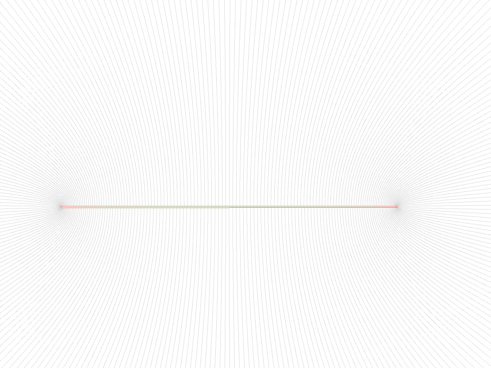
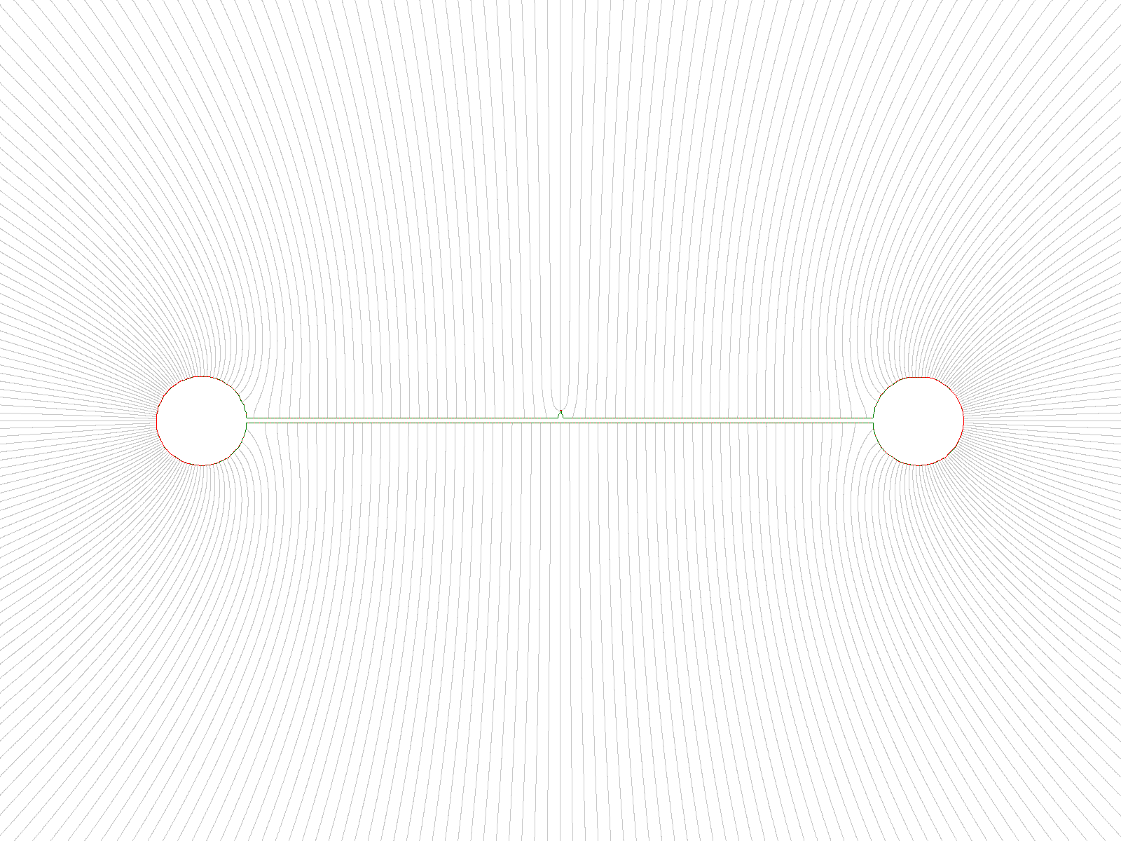
The program will stop automatically when charge movement
drops below a threshold. When the program stops, a PNG file with field lines is
written to the output directory.
Press Ctrl+C to stop the program early. The program will
write a PNG file with field lines for the current state of the model.
While using the snapshot PNG files to monitor the charge
distribution progress is useful for debugging, it does not accurately reflect
electron movement in a read conductor. Only when the model reaches equilibrium
do its charges match the behavior of electrons in a conductor. When the charges
in this simulation are redistributing, a charge can quickly move across the
entire length of the conductor. We know this doesn’t happen in real conductors.
For example, when an electrical pulse travels over miles of wire at the speed of
light, no single electron moves from one end of the wire to the other at the
speed of light. So while it is fun to watch the motion of the charges in the
simulation, it is important to remember real electrons don’t move this way.
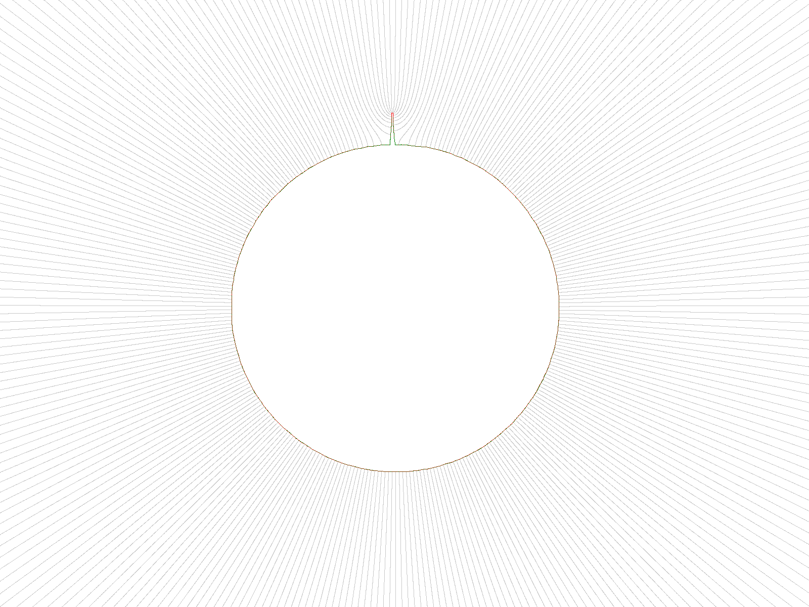
Another difference between this model and a real conductor
is that the model is 2D and a real conductor is 3D. The 2D conductors in the
simulation represent a slice of a 3D conductor that extends indefinitely. A 2D
circle model corresponds a 3D cylinder of infinite length. A 2D triangle model
corresponds to a 3D prism of infinite length.